Regularization
Regularization is the art of preventing overfitting by adding constraints to the learning process. It's one of the most important concepts in machine learning.
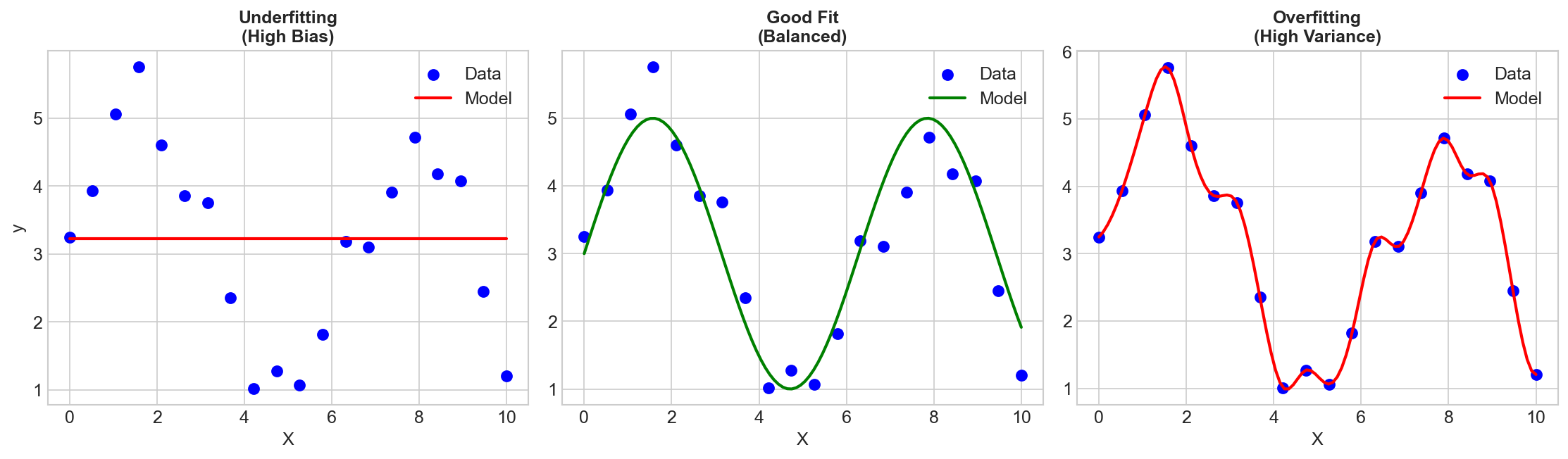
Why Regularize?
Models can fit training data too well, capturing noise instead of signal. Regularization adds a penalty for complexity:
Total Loss = Training Loss + λ × Complexity Penalty
Where λ controls the regularization strength.
L2 Regularization (Ridge)
The Penalty
Penalty = λ × Σ wᵢ²
Adds the squared magnitude of weights to the loss.
Effect
- Shrinks weights toward zero (but not exactly to zero)
- Larger weights penalized more heavily
- Weights distributed across features
Mathematical View
Equivalent to:
- Constraining ||w||² ≤ t
- Assuming Gaussian prior on weights (Bayesian view)
When to Use
- When most features are useful
- Don't need feature selection
- Default choice for many problems
L1 Regularization (Lasso)
The Penalty
Penalty = λ × Σ |wᵢ|
Adds the absolute value of weights to the loss.
Effect
- Drives some weights exactly to zero
- Automatic feature selection
- Produces sparse models
Why Sparsity?
The L1 constraint forms a diamond shape in weight space. Optimal points are likely to hit corners (where some weights are zero).
When to Use
- When you suspect many features are irrelevant
- Want interpretable sparse models
- Feature selection is important
L1 vs L2 Comparison
| Aspect | L1 (Lasso) | L2 (Ridge) |
|---|---|---|
| Penalty | Sum of | wᵢ |
| Sparsity | Yes | No |
| Feature selection | Automatic | No |
| Correlated features | Picks one | Spreads weight |
| Stability | Less stable | More stable |
| Solution | Not always unique | Unique |
Elastic Net
Combines L1 and L2:
Penalty = α × L1 + (1-α) × L2
Gets sparsity from L1 and stability from L2.
Best of both worlds for correlated features.
Regularization in Different Models
Linear/Logistic Regression
- Ridge, Lasso, or Elastic Net
- Controlled by λ (alpha in sklearn)
Decision Trees
- Max depth
- Min samples per leaf
- Pruning
Neural Networks
- Weight decay (L2 on weights)
- Dropout
- Batch normalization (implicit)
- Early stopping
SVMs
- C parameter (inverse of λ)
- Lower C = more regularization
Modern Regularization Techniques
Dropout
Randomly zero out neurons during training.
- Prevents co-adaptation
- Ensemble effect
- See: Dropout concept
Batch Normalization
Normalizes layer inputs.
- Implicit regularization effect
- Allows higher learning rates
Data Augmentation
Create modified versions of training data.
- Rotations, flips, crops for images
- Paraphrasing for text
- Implicitly adds invariances
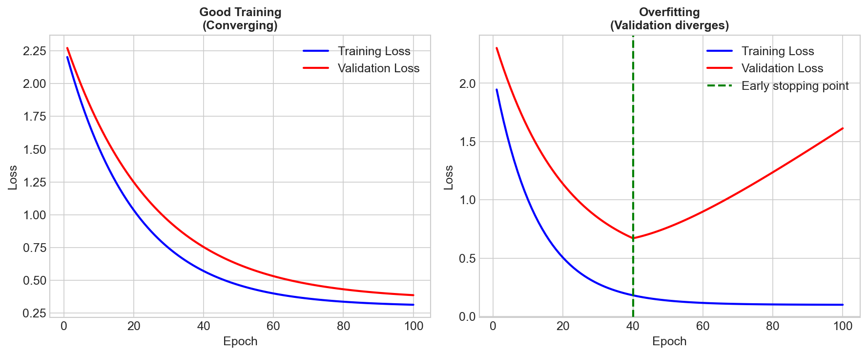
Early Stopping
Stop training before convergence.
- Monitor validation loss
- Implicit regularization
- Simple but effective
Choosing Regularization Strength
Cross-Validation
The gold standard:
- Try several λ values
- Evaluate each with CV
- Pick λ with best validation score
Learning Curves
Plot train/validation error vs λ:
- High λ: Both errors high (underfitting)
- Low λ: Training low, validation high (overfitting)
- Sweet spot: Where validation error is minimized
The Bayesian Perspective
Regularization is equivalent to placing priors on weights:
| Regularization | Prior |
|---|---|
| L2 | Gaussian (mean 0) |
| L1 | Laplace (double exponential) |
| None | Uniform (improper) |
Maximum A Posteriori (MAP) estimation with these priors gives regularized solutions.
Common Pitfalls
-
Regularizing the bias: Usually don't regularize the intercept/bias term
-
Not scaling features: With L1/L2, larger-scale features are penalized more. Standardize first!
-
Same λ for all features: Sometimes different features need different regularization
-
Over-regularizing: Can cause underfitting
Key Takeaways
- Regularization prevents overfitting by penalizing complexity
- L2 (Ridge): Shrinks weights, keeps all features
- L1 (Lasso): Produces sparse models, feature selection
- Elastic Net: Combines L1 and L2
- Always cross-validate to choose regularization strength
- Neural networks use dropout, batch norm, weight decay