Bias-Variance Tradeoff
The bias-variance tradeoff is one of the most important concepts in machine learning. It explains why models fail and guides us toward better solutions.
The Decomposition
The expected prediction error can be decomposed into three parts:
Error = Bias² + Variance + Irreducible Noise
Bias
Error from wrong assumptions in the model.
- High bias = model is too simple
- Can't capture the true relationship
- Leads to underfitting
Variance
Error from sensitivity to training data fluctuations.
- High variance = model is too complex
- Captures noise in training data
- Leads to overfitting
Irreducible Noise
Inherent randomness in the data that no model can explain.
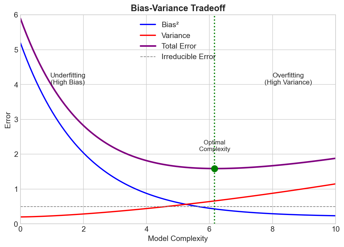
The Tradeoff
As model complexity increases:
- Bias decreases: More flexible models fit better
- Variance increases: More sensitive to training data
The goal is finding the sweet spot where total error is minimized.
Simple Model ←————————————————→ Complex Model
High Bias                          High Variance
Low Variance                       Low Bias
Underfitting                       Overfitting
Visual Intuition
Imagine fitting a curve to noisy data:
-
Linear model (high bias): Straight line can't capture curves. Consistently wrong.
-
Very complex polynomial (high variance): Wiggles through every point. Different training sets give wildly different curves.
-
Moderate polynomial (balanced): Captures the general trend without fitting noise.
Diagnosing the Problem
High Bias (Underfitting)
- Training error is high
- Training and validation error are similar
- Model performs poorly everywhere
Solutions:
- Use more complex model
- Add more features
- Reduce regularization
- Train longer (for neural nets)
High Variance (Overfitting)
- Training error is low
- Validation error is much higher than training
- Large gap between train and validation
Solutions:
- Get more training data
- Use simpler model
- Add regularization (L1, L2, dropout)
- Use ensemble methods
- Early stopping
Model Complexity Examples
| Model | Typical Bias | Typical Variance |
|---|---|---|
| Linear Regression | High | Low |
| Decision Tree (deep) | Low | High |
| Random Forest | Low | Lower (ensembled) |
| Neural Net (large) | Low | High |
| k-NN (k=1) | Low | High |
| k-NN (k=large) | High | Low |
Regularization's Role
Regularization explicitly controls the tradeoff:
Loss = Training Error + λ × Complexity Penalty
- λ = 0: No regularization, risk overfitting
- λ = large: Heavy penalty, risk underfitting
- λ = optimal: Balances bias and variance
The Modern Deep Learning Twist
Classical theory suggests very large neural networks should overfit terribly. But in practice:
- Double descent: Error can decrease again with very large models
- Implicit regularization: SGD and architecture choices act as regularizers
- Interpolation regime: Models that perfectly fit training data can still generalize
This is an active area of research that challenges traditional understanding.
Ensemble Methods
Ensembles reduce variance without increasing bias:
- Bagging (Random Forest): Average multiple high-variance models
- Boosting (XGBoost): Sequentially reduce bias
This is why ensembles often work so well.
Key Takeaways
- Error = Bias² + Variance + Noise
- More complexity: lower bias, higher variance
- Underfitting → reduce bias; Overfitting → reduce variance
- Regularization controls the tradeoff
- Ensembles can reduce variance without adding bias
- Modern deep learning challenges classical theory