Confusion Matrix
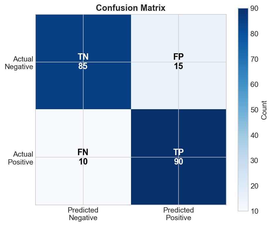
A confusion matrix is a table that describes the performance of a classification model by showing actual vs. predicted classes. It's the foundation for computing most classification metrics.
Binary Classification
For two classes (Positive/Negative):
                    Predicted
                 Positive  Negative
         Pos       TP        FN
Actual
         Neg       FP        TN
| Cell | Name | Meaning |
|---|---|---|
| TP | True Positive | Correctly predicted positive |
| TN | True Negative | Correctly predicted negative |
| FP | False Positive | Incorrectly predicted positive (Type I error) |
| FN | False Negative | Incorrectly predicted negative (Type II error) |
Reading the Matrix
Example: Disease Detection
                    Predicted
                  Disease  Healthy
         Disease    85       15      (100 actual diseased)
Actual
         Healthy    10       890     (900 actual healthy)
                   (95)     (905)
Interpretation:
- 85 patients correctly identified as having disease (TP)
- 15 patients with disease missed (FN) - dangerous!
- 10 healthy patients incorrectly told they have disease (FP)
- 890 healthy patients correctly identified (TN)
Metrics from Confusion Matrix
Accuracy
Accuracy = (TP + TN) / (TP + TN + FP + FN)
         = (85 + 890) / 1000 = 97.5%
Overall correctness.
Precision (Positive Predictive Value)
Precision = TP / (TP + FP)
          = 85 / 95 = 89.5%
"When we predict positive, how often are we right?"
Recall (Sensitivity, True Positive Rate)
Recall = TP / (TP + FN)
       = 85 / 100 = 85%
"Of actual positives, how many did we catch?"
Specificity (True Negative Rate)
Specificity = TN / (TN + FP)
            = 890 / 900 = 98.9%
"Of actual negatives, how many did we correctly identify?"
F1 Score
F1 = 2 × (Precision × Recall) / (Precision + Recall)
   = 2 × (0.895 × 0.85) / (0.895 + 0.85) = 87.2%
Harmonic mean of precision and recall.
Multi-class Confusion Matrix
Extends to N classes (N×N matrix):
                      Predicted
               Cat    Dog    Bird
       Cat     45      3      2      (50)
Actual Dog      4     38      8      (50)
       Bird     2      5     43      (50)
               (51)   (46)   (53)
Reading Multi-class
- Diagonal: Correct predictions
- Off-diagonal: Confusion between classes
- Row totals: Actual counts per class
- Column totals: Predicted counts per class
Common Patterns
Dog confused with Cat (row Dog, col Cat = 4):
- 4 dogs were predicted as cats
- Model might struggle with similar features
Cat well-predicted (row Cat, col Cat = 45):
- 45/50 = 90% recall for cats
Per-class Metrics
Compute precision, recall for each class:
# Cat metrics
Precision_cat = 45 / 51 = 88.2%  # TP / column total
Recall_cat = 45 / 50 = 90%        # TP / row total

# Similarly for Dog, Bird...
Normalized Confusion Matrix
Normalize rows to see percentages:
                      Predicted
               Cat    Dog    Bird
       Cat    90%     6%     4%
Actual Dog     8%    76%    16%
       Bird    4%    10%    86%
Easier to spot which classes are confused.
Visualizing Confusion Matrices
import seaborn as sns
from sklearn.metrics import confusion_matrix, ConfusionMatrixDisplay

# Generate matrix
cm = confusion_matrix(y_true, y_pred)

# Plot
disp = ConfusionMatrixDisplay(cm, display_labels=['Cat', 'Dog', 'Bird'])
disp.plot(cmap='Blues')
Heatmap tips:
- Use color intensity for magnitude
- Normalize for class imbalance
- Include both counts and percentages
What Confusion Patterns Tell You
Balanced Diagonal
[95,  5]     Model works well,
[ 4, 96]     balanced performance
High FP (Column > Row)
[80, 20]     Predicts positive too often,
[40, 60]     many false alarms
May need higher threshold or more negative training data.
High FN (Row > Column)
[60, 40]     Misses many positives,
[ 5, 95]     under-predicting
May need lower threshold or more positive training data.
Class Confusion
[80,  2, 18]     Classes 0 and 2 confused,
[ 1, 95,  4]     consider feature engineering
[15,  3, 82]     or more training data
Imbalanced Classes
Confusion matrix reveals imbalance effects:
               Pred+  Pred-
Actual+         5      5      (10 positives = 1%)
Actual-        10    985      (990 negatives = 99%)
- Accuracy = 990/1000 = 99% (misleading!)
- Recall = 5/10 = 50% (missing half the positives!)
Always look at the matrix, not just accuracy.
Practical Tips
- Always examine the matrix before trusting a single metric
- Normalize by rows for class-balanced view
- Sort classes by confusion to spot patterns
- Compare matrices at different thresholds
- Log misclassified examples for error analysis
Code Example
from sklearn.metrics import (
    confusion_matrix,
    classification_report
)

# Generate matrix
cm = confusion_matrix(y_true, y_pred)
print(cm)

# Full report with all metrics
print(classification_report(y_true, y_pred))
Output:
              precision    recall  f1-score   support

         Cat       0.88      0.90      0.89        50
         Dog       0.83      0.76      0.79        50
        Bird       0.81      0.86      0.84        50

    accuracy                           0.84       150
   macro avg       0.84      0.84      0.84       150
Key Takeaways
- Confusion matrix shows actual vs predicted for all classes
- Diagonal = correct, off-diagonal = errors
- Enables computing precision, recall, F1 per class
- Reveals class confusion patterns
- Essential for imbalanced data analysis
- Always visualize before trusting single metrics