Principal Component Analysis (PCA)
PCA is the most widely used dimensionality reduction technique. It transforms data into a new coordinate system where the axes (principal components) capture maximum variance.
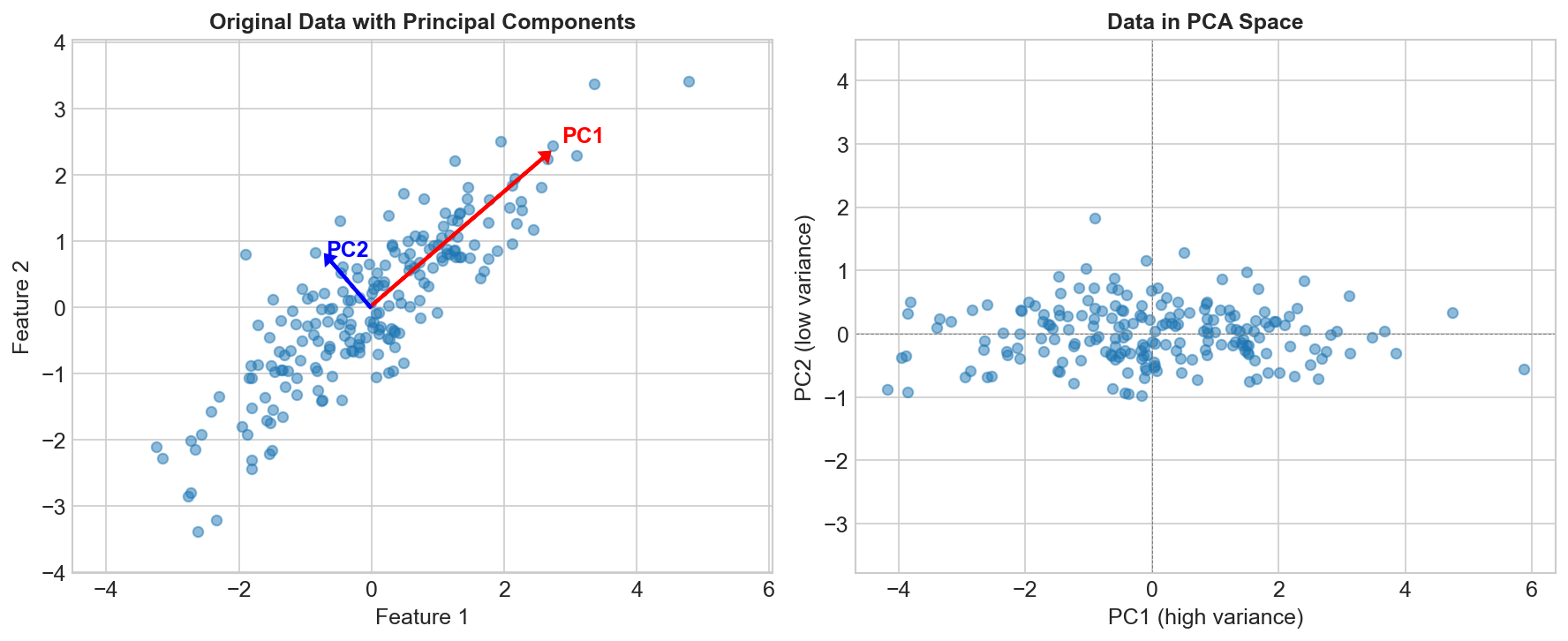
The Core Idea
Find directions (principal components) that:
- Capture maximum variance in the data
- Are orthogonal (perpendicular) to each other
- Are ordered by variance explained
Original 2D data:        After PCA:
    •  •                    PC1 →
   •  •  •                 •  •  •  •
  •  •  •  •               •  •  •
   •  •  •                   ↑
    •  •                    PC2
The Algorithm
Step 1: Center the Data
X_centered = X - mean(X)
Step 2: Compute Covariance Matrix
Σ = (1/n) × Xᵀ × X
Step 3: Find Eigenvectors and Eigenvalues
Σv = λv

Eigenvectors = principal component directions
Eigenvalues = variance explained by each component
Step 4: Sort and Select
Sort eigenvectors by eigenvalue (descending)
Keep top k components
Step 5: Transform
X_reduced = X_centered × W

Where W = [v₁, v₂, ..., vₖ] (top k eigenvectors)
Variance Explained
Individual Component
Variance explained by PCᵢ = λᵢ / Σλⱼ
Cumulative Variance
Cumulative = Σᵢ₌₁ᵏ λᵢ / Σλⱼ
Often keep components that explain 95% of variance.
Choosing Number of Components
Scree Plot
Plot eigenvalues, look for "elbow":
Variance
    |\
    | \
    |  \__
    |     \___
    |_________
         PC
Cumulative Variance Threshold
pca = PCA(n_components=0.95) # Keep 95% of variance
Kaiser Criterion
Keep components with eigenvalue > 1 (when using correlation matrix).
PCA Properties
What PCA Does
- Decorrelates features
- Orders by importance (variance)
- Reduces dimensionality
- Can reveal hidden structure
What PCA Doesn't Do
- Consider class labels (unsupervised)
- Guarantee better classification
- Handle non-linear relationships
- Work well with categorical data
When to Use PCA
Good for:
- Visualization (reduce to 2-3 dimensions)
- Noise reduction (remove low-variance components)
- Feature decorrelation
- Speeding up other algorithms
- Handling multicollinearity
Not good for:
- When all features are important
- Non-linear relationships (use kernel PCA)
- When interpretability is crucial
- Sparse data (use TruncatedSVD)
Practical Considerations
Scaling
from sklearn.preprocessing import StandardScaler

# ALWAYS scale before PCA!
X_scaled = StandardScaler().fit_transform(X)
pca.fit(X_scaled)
PCA is sensitive to scale. Standardize first!
Interpreting Components
# Component loadings (how much each feature contributes)
components = pca.components_  # Shape: (n_components, n_features)

# PC1 = 0.5*feature1 + 0.3*feature2 - 0.4*feature3 + ...
Reconstruction
# Transform to lower dimension
X_reduced = pca.transform(X_scaled)

# Reconstruct (with some loss)
X_reconstructed = pca.inverse_transform(X_reduced)

# Reconstruction error
error = np.mean((X_scaled - X_reconstructed)**2)
Code Example
from sklearn.decomposition import PCA
from sklearn.preprocessing import StandardScaler
import matplotlib.pyplot as plt

# Scale data
scaler = StandardScaler()
X_scaled = scaler.fit_transform(X)

# Fit PCA
pca = PCA(n_components=0.95)  # Keep 95% variance
X_reduced = pca.fit_transform(X_scaled)

print(f"Original dimensions: {X.shape[1]}")
print(f"Reduced dimensions: {X_reduced.shape[1]}")
print(f"Variance explained: {pca.explained_variance_ratio_}")

# Plot cumulative variance
plt.plot(np.cumsum(pca.explained_variance_ratio_))
plt.xlabel('Number of Components')
plt.ylabel('Cumulative Variance Explained')
PCA vs Other Methods
| Method | Linear | Supervised | Use Case |
|---|---|---|---|
| PCA | Yes | No | General dim reduction |
| LDA | Yes | Yes | Classification |
| t-SNE | No | No | Visualization |
| UMAP | No | No | Visualization + structure |
| Autoencoders | No | No | Complex patterns |
Kernel PCA
For non-linear relationships:
from sklearn.decomposition import KernelPCA

kpca = KernelPCA(n_components=2, kernel='rbf')
X_kpca = kpca.fit_transform(X)
Maps to higher dimension, then applies PCA.
Key Takeaways
- PCA finds orthogonal directions of maximum variance
- Principal components are eigenvectors of covariance matrix
- Always standardize features before PCA
- Keep enough components to explain ~95% variance
- Good for visualization, denoising, and preprocessing
- Use kernel PCA for non-linear patterns